Contents

1 Introduction

Aurora is a particle tracking partner for MODFLOW-2005 (and MODFLOW-2000, although this is less thoroughly tested) to model solute transport at field scale. Aurora works by performing continuous-time random walk (CTRW) particle tracking on groundwater flow fields determined by MODFLOW. As a particle tracker, it is free of the numerical dispersion and instability inherent in Eulerian transport codes. It also offers richer transport physics than are available in other solute transport codes that work with MODFLOW, such as the MODPATH and MT3D families. Some features of the Aurora software:

• \(\blacksquare \) It can model classical advection and dispersion as well as non-Fickian transport models including any physics that can be captured by CTRW or time-fractional advection-dispersion approaches.

• \(\blacksquare \) It can model all multi-rate mass transfer processes, as well as capturing classical first-order kinetic sorption and the retardation coefficient approximation.

• \(\blacksquare \) It can capture arbitrarily-complex multi-species first-order decay networks with arbitrary stoichiometry.

• \(\blacksquare \) It can implement multiple types of solute sources, including time-varying specified concentration, time-varying specified injection rate, and raw particle injection (with and without flux weighting, as desired).

• \(\blacksquare \) It can record solute particle locations at arbitrary times and breakthroughs at arbitrary planes and curved surfaces.

Aurora is, to our knowledge, the only full-physics particle tracker for groundwater transport problems and the only software, regardless of numerical approach, to model general non-Fickian subsurface transport. The combination of MODFLOW and Aurora enables a natural and practical approach to modeling solute transport at the field scale: deterministic, explicitly resolved flow information from MODFLOW is used directly while unresolved small-scale physical and chemical heterogeneity that may cause non-Fickian transport is captured by Aurora’s stochastic particle tracking. In general, any behaviour that can be captured by the classical advection-dispersion equation (ADE), or by the more general CTRW framework (which includes multi-rate mass transfer and any behavior captured by the time-fractional ADE), can be modeled by Aurora.

The output of Aurora consists of listings of particle locations (recorded at user-specified times), and listings of times of particle arrivals (recorded at user-specified planes). These can be visualized as plume movies and stills and breakthrough curves using included visualization Python scripts, which apply kernel density estimation to reconstruct plume concentrations, or by any other post-processing software.

2 How Aurora works

2.1 Basic theory

Aurora interpolates the cell-to-cell flows computed by MODFLOW to determine the implied groundwater velocity at each point in space, and the implied streamlines of the large-scale groundwater flow. Transport of dissolved chemicals or colloids is simulated by tracking particles along these streamlines, as they make steps of fixed length but random duration along these streamlines. We refer to this approach as CTRW-on-a-streamline: a 1D CTRW is performed on a curved path in 3D. Because the spatial steps size is fixed, this may also be considered a time-domain random walk. When using Aurora to capture groundwater transport, the goal is to choose the probability distribution describing the random step time in such a way as to correspond to real physics. The theoretical discussion in Section 5 assists with this. Here, we briefly introduce the algorithm but avoid going into great detail.

In a CTRW particle tracking scheme, each particle is represented as a spatial location and a time, both of which are updated iteratively. At iteration \(n\), position \(\bm {x}_n\ \mathrm {[L]}\), and clock time \(t_{C,n}\ \mathrm {[T]}\) are updated according to the following equations:

\begin{eqnarray} \bm {x}_{n+1} &=& \bm {x}_n + \frac {\bm {v}(\bm {x}_n)}{\| \bm {v}(\bm {x}_n) \|}d + \Delta _{\bm {x},n} \label {eq: space update formal}\\ t_{C,n+1} &=& t_{C,n} + \Delta _{t_C,n}. \label {eq: time update formal} \end{eqnarray}

\(\bm {x}_n\) is updated by traveling \(d\ \mathrm {[L]}\) units along the local streamline, and then making a random jump, \(\Delta _{\bm {x},n}\ \mathrm {[L]}\) in the plane orthogonal to \(\bm {v}(\bm {x}_n)\ \mathrm {[LT^{-1}]}\), each of whose components is drawn from \(\mathcal {N}(0,2 \alpha _t d)\), where \(\alpha _t\ \mathrm {[L]}\) is the medium’s transverse dispersivity. The time increment, \(\Delta _{t_C,n}\ \mathrm {[T]}\), is specified via two functions and one parameter chosen by the user:

\(\bm {f(r)}\):

a probability density function (pdf) representing the ratio of \(\Delta _{t_A,n}\ \mathrm {[T]}\), the actual time taken for advection from \(\bm {x}_n\) to \(\bm {x}_{n+1}\), accounting for all advective heterogeneity, to \(d/\| \bm {v}(\bm {x}_n) \|\), the time taken when accounting only for large-scale heterogeneity. For the large scale velocity field to be on average correct, this distribution must be chosen so that \(\mathrm {E}[r]=1\). Several distributions for \(f(r)\) are presently implemented in Aurora: shifted Dirac (i.e., pure streamline tracing), inverse Gaussian (i.e., ADE behavior), Log-normal, Pareto, and TPL. Dimensionless.

\(\bm {\lambda }\):

the probability of immobilization of any given particle per unit time. Units \(\mathrm {[T^{-1}]}\).

\(\bm {g(t)}\):

a pdf representing the amount of time a particular particle remains immobilized during a given immobilization event. Exponential and tempered power law models are available. Units \(\mathrm {[T^{-1}]}\).

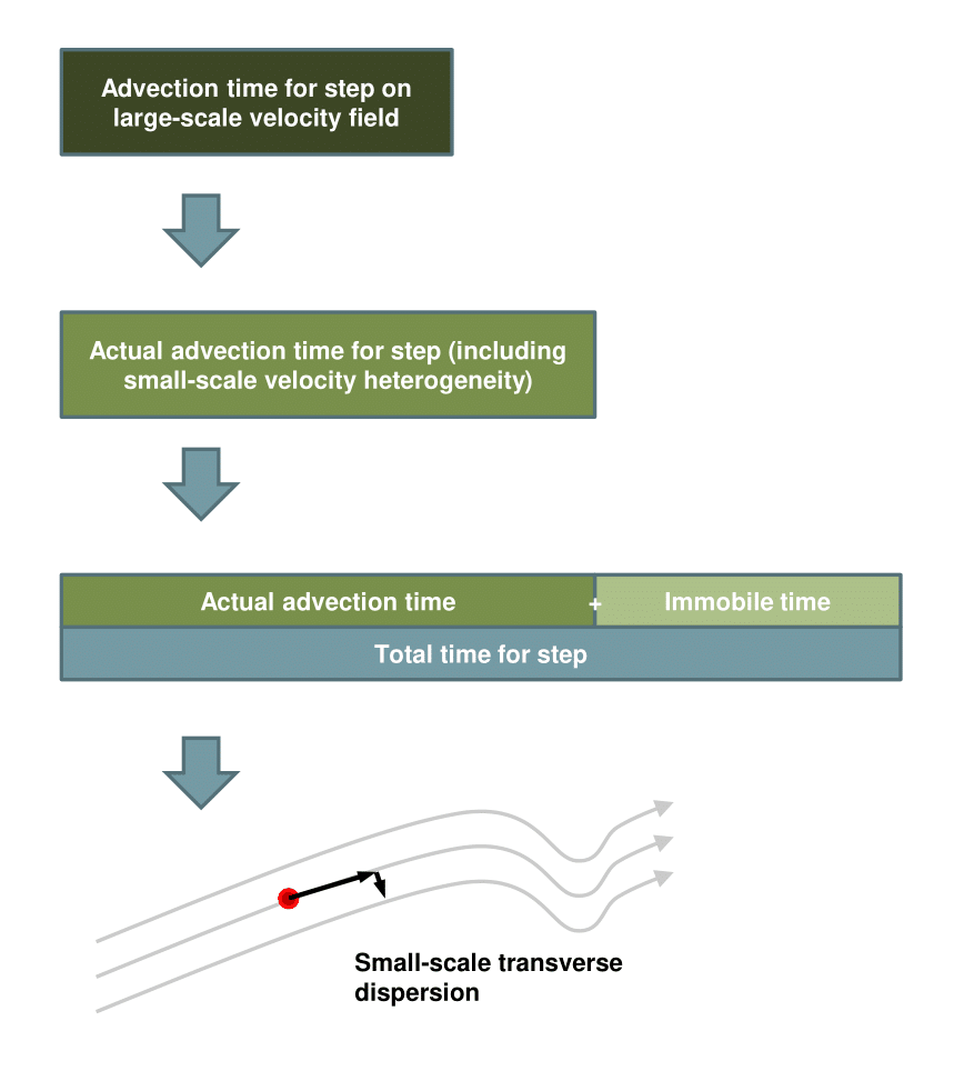
\(\Delta _{t_A,n}\) is computed by drawing randomly from \(f(r)\) and multiplying by \(d/\| \bm {v}(\bm {x}_n) \|\) to compute \(\Delta _{t_A,n}\). Then a number of immobilization events, \(i\), is selected by drawing randomly from \(\mathrm {Poisson}(\lambda \Delta _{t_A,n})\). For each step of each particle, \(n\) draws from \(g(t)\) are performed, summed, and then added to arrive at \(\Delta _{t_C,n}\). Once the step is completed, a random motion representing local-scale Fickian dispersion is added in a plane orthogonal to \(\bm {v}(\bm {x}_n)\). The strength of this transverse dispersion is specified by a user-defined dispersivity, \(\alpha _t\). The particle tracking process is summarized in Figure 1. All user-specified parameters are assumed to apply uniformly in each layer, but may differ between them.

2.2 The Aurora coordinate system and the MODFLOW grid

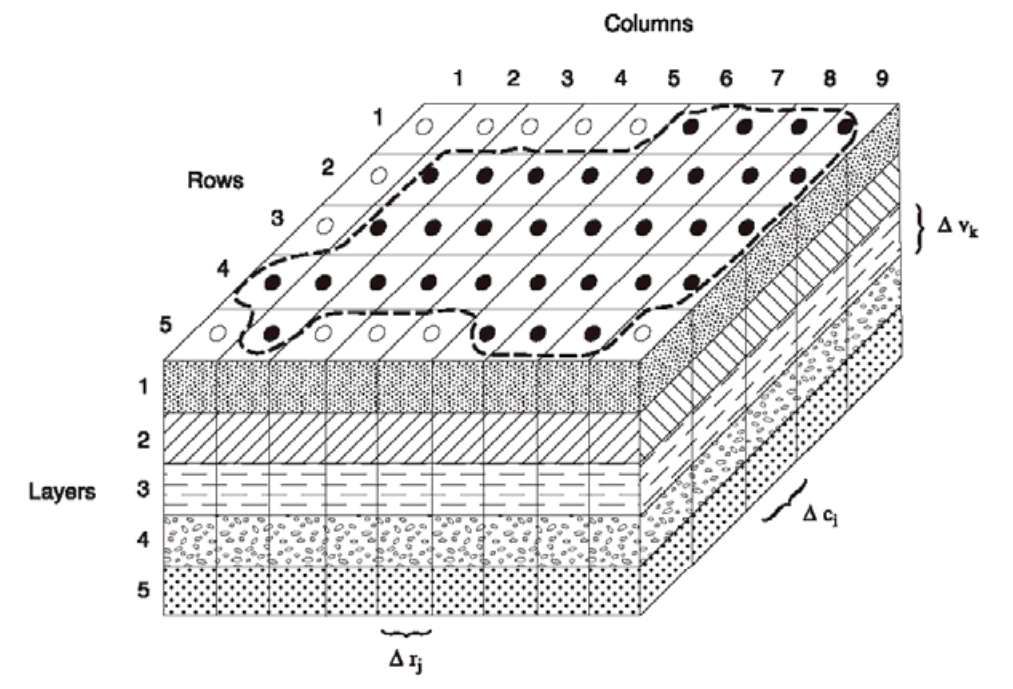
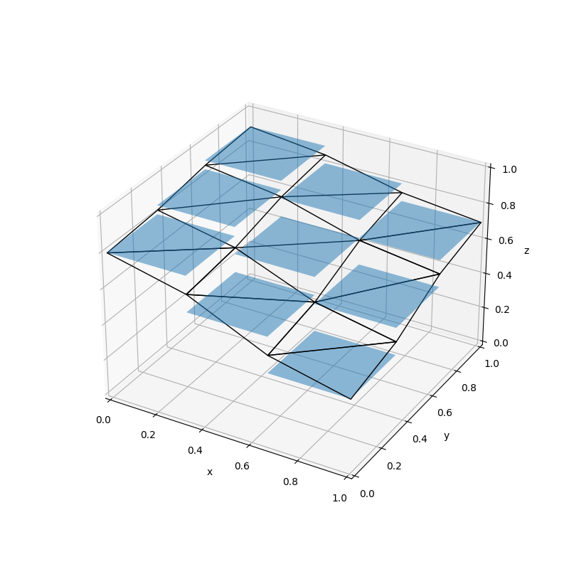
As a particle tracker, Aurora works in continuous \(x,y,z-\)coordinates. By contrast, MODFLOW is a finite difference code that operates on a 3D structured grid with shoebox-shaped volumes. In addition, while a MODFLOW domain is a perfect grid in map view, the vertical elevations of cell interfaces are permitted to change from cell-to-cell to follow stratigraphy. This leads to layer discontinuities at vertical cell interfaces. Figure 2 illustrates the discretization of a MODFLOW model into potentially vertically staggered volumes. However, in the mathematical formulation, horizontal hydraulic connectivity only exists between cells in the same layer. Put another way, MODFLOW only allows water to flow between cells if only one of their row, column, or layer indexes differ by one and their other indexes are identical. Aurora resolves these matters by treating upper and lower layer boundaries as though they are defined by continuous interpolating surfaces constructed by tessellating triangular planes, and localizing particles in their appropriate layer relative to these surfaces. The location of this these interfaces is computed in the following way: for each layer of cells, for each node where cell corners are found in the \(x'\)-\(y'\) plane, the elevation of the cell tops (either 1, 2, or 4 cells are used depending on where the node is located on the boundary) is averaged. This quantity is taken to be the true elevation of the layer’s upper interface at the corresponding point \((x',y')\) These elevations are joined by straight line segments along the cell boundaries in the the \(x'\)-\(y'\) plane. For each cell, another line segment is placed that divides its top into two equally-sized right-angle triangles when viewed from directly above. In this way, the entire model domain is crossed by a triangular tessellation that is continuous (because each edge of each triangle is co-linear with the corresponding edge of each of its neighbours) and which well approximates the interface. An identical procedure is performed, using the cell bottoms of the bottom layer to interpolate the domain bottom. If an interface is flat, this tessellation will exactly match it, and where it features discontinuities, this surface will interpolate it in an unbiased way. Figure 3 illustrates the procedure.

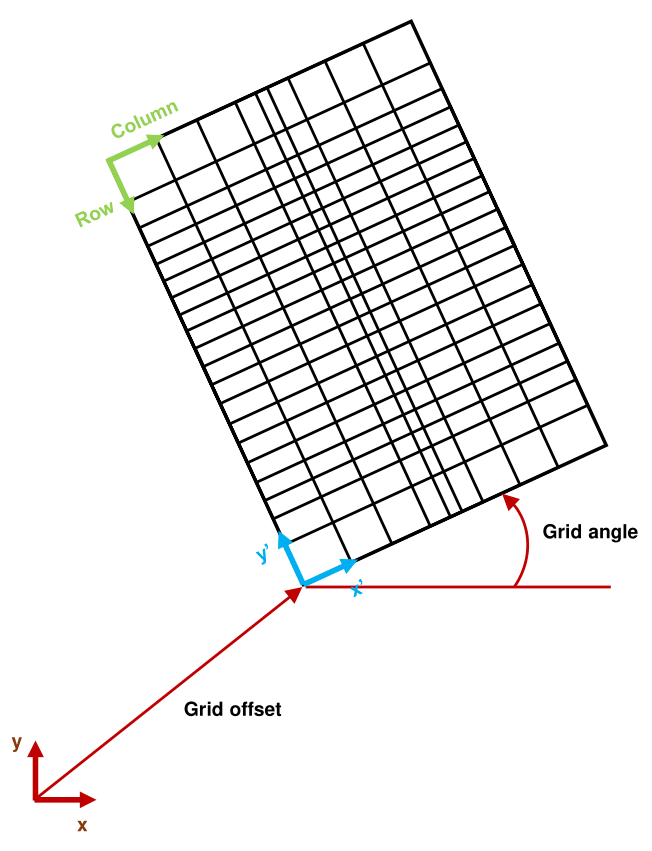
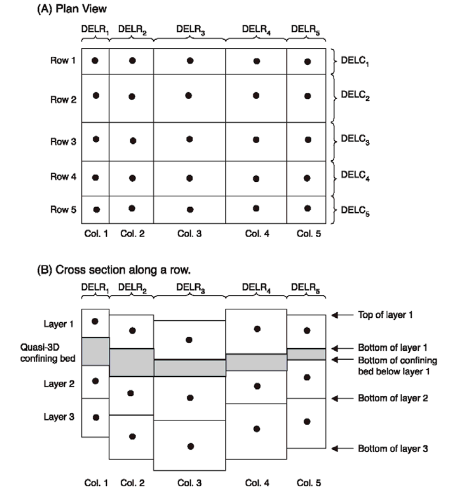
It is also important to understand the relationship between the MODFLOW discretization and the coordinate system used by Aurora. As seen in Figure 2, MODFLOW indexes its rows and columns in the standard fashion for matrix indexes, and its layer indexes increase with increasing depth. Aurora internally uses a \(x',y',z\) coordinate system with standard right hand rule chirality. Its origin is at the bottom lower left of the domain shown in Figure 2, which is to say at the bottom of the lowest layer, at the end of the highest-index row, and at the start of the lowest-index column. \(x'\) increases with increasing column index, \(y'\) increases with decreasing row index, and \(z\) increases with decreasing layer index (i.e., it points upwards). For convenience, the user may work in any coordinate system in the Aurora marshal file, so long as it also features standard right hand rule chirality and features an upward-directed \(z\) axis (parallel to the one used internally). This is likely confusing, so Figure 4 shows the inter-relation of all of the indexing systems.

Naturally, it is necessary for Aurora to know the offset of the origin of the internal coordinate system from the origin of the system used in the marshal file, as well as the grid angle (in degrees) of the \(x'\)-axis relative to the \(x\)-axis. Otherwise, it would not be possible to relate the \(x,y,z\) particle position to a corresponding location in the MODFLOW domain and thereby infer its streamline velocity. This may be done in a number of ways. It is possible to manually specify grid angle and offset in the marshal file. It is also possible to specify that this is to be selected automatically, in which case Aurora looks for a ModelMuse comment at the top of the .dis file indicating model boundary coordinates and grid angle. If this is not found, Aurora defaults to zero grid angle and zero offset, effectively identifying \(x,y,z\) and \(x',y',z\) coordinates.

2.3 Computing velocities from water budgets and levels

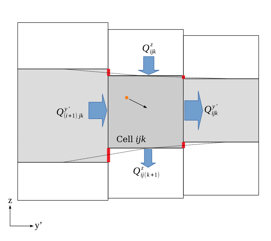
Aurora computes the groundwater velocity at any needed location in the domain by processing and interpolating water budget data produced by MODFLOW. MODFLOW reports the rate at which water is transferred from each cell to its neighbours through each of the cell’s faces for each time step. By dividing the volumetric flow rate through a given face by its saturated cross-sectional area, Aurora is able to obtain the average Darcy flux through each face. This is trilinearly interpolated using the so-called Pollock method: the Darcy flux component in the \(x'\) direction at some location within a cell is determined by linear interpolation of the average Darcy fluxes through each of the two cell faces orthogonal to an \(x'\)-directed vector. A similar procedure is used to infer the \(y'\)- and \(z\)-directed Darcy flux components. This flux vector is converted into a velocity vector by dividing all components by the porosity of the cell (as implemented, all cells in a layer share a porosity, but it can differ between layers). This interpolation is illustrated in 2D in Figure 5.

For all purposes, the layer interfaces defined by the triangular tessellations shown in Figure 3 are taken to be the real upper and lower boundaries of each cell. This means that the layer whose budgets and porosity apply to a given particle are determined by its position relative to the tessellations, even if straightforwardly mapping its location onto the “shoebox” voxels of the *.dis file would put it in a neighbouring layer. This is done for consistency with transport behavior at the top and bottom of the domain. Furthermore, the facial cross-sectional area is computed based on the area between the top and bottom tessellations, not from the raw area computed from the discretization file. This ensures continuity of velocity through all cell interfaces and conceptual consistency.

Where layers are sloping, an additional vertical velocity component is added when computing the velocities implied by horizontal (i.e., within layer) fluxes, so that the particle’s relative height within the layer is preserved (i.e., it relative vertical position between the upper and lower layer interface tessellations). The need for this can be seen by imagining a system with a single, sloped layer. Because all fluxes are within-layer, naive interpolation would lead only to horizontal components of velocity, causing particles to advect out of model bounds when actually any flow at the top and bottom of the model must be parallel to the (impermeable) boundaries. The same behaviour should then hold in multiple layer systems for consistency.

If a cell is wholly saturated, it is possible for Aurora to compute velocities within using only geometric information. However, if the water table drops so that it bisects a cell face, it is only appropriate to use the area below the water table for computing the average Darcy flux that is interpolated—we assume there is no transport in the vadose zone. Use of the whole interfacial area will result in underestimation of the velocity. Using head information from MODFLOW, the location of the water table is computed for each cell. The water table is interpolated in exactly the same fashion as the cell interfaces, by means of a triangular tessellation. (One water table level computation is made for each layer of the domain, so it is possible to have perched aquifers; a given layer’s water table surface only impacts velocity computation if and when it intersects cells in the same layer.) If the water table intersects a face, the exact area of the face below the water table is computed and this is used for computing the average Darcy flux through that face.

Because transport is considered not to occur above the water table, the water table behaves locally like the top of the model. If advective or dispersive motion acts to move a particle above the water table, it is reflected so that it remains in the domain, beneath the water table. Aurora checks between any particle motions whether the particle is below the water table and takes appropriate action, so it is never possible for particles to become stuck in a dry region, or for the particle tracker to ask for a velocity in a region in which it is undefined.

2.4 Sources

Solute sources must be specified in order for any particles to be introduced into the domain. Every source is associated with a region of the domain, which may have a variety of primitive geometric shapes, including boxes (parallelepipeds), spheres, cylinders, and cylindrical shells. Particles are introduced at random locations in the interior or surface of these shapes, either uniformly or proportionally to local Darcy flux components, depending on source specification. The time at which individual particles are introduced depends on the type of the source, described below.

2.4.1 Raw particle source

The simplest type of source is a “raw” source, in which particles are introduced without regard for the concentration of other particles nearby. A user-specified number of particles are introduced at a single instant, or uniformly randomly between two fixed times. The initial location of each particle is random within the source region: either uniformly random (all locations in the region are equally likely), or randomly drawn from a distribution that is proportional to the magnitude of the Darcy flux at each location in the region.

2.4.2 Specified molar concentration source

Molar concentration sources allow the molar concentration within the source region to be set to a constant value throughout each of one or more epochs: corresponding to a type I or Dirichlet boundary condition on an Eulerian perspective. The user must define the number of moles per particle and the target molar concentration. If this will result in under 50 particles in some source, Aurora will automatically increase the number of particles in that source to 50 and randomly eliminate (but replace) a proportion of those exiting the source so that the specified moles-per-particle ratio is still upheld in the domain. For each fixed-concentration epoch, the correct number of particles to be maintained in the source region is calculated, and these are initialized at uniformly random spatial locations throughout the region at the start time of the epoch. For clarity, separate sets of particles are initialized for each epoch.

During the active epochs of the source, the appropriate concentration is maintained by monitoring particle transitions of particles of the same species as the source that are associated with the source region. The following actions are taken on completion of transition of particles of the same species as an active source:

• 1. Eliminate any particles that transition into the source region.

• 2. Replace any particles that transition out of the source with another particle of the same species, spawned at a random location within the region at the time of the exiting particle’s departure.

• 3. Eliminate particles remaining within the source region whose clock time crosses the transition time between two fixed-concentration epochs. (The correct number of particles to set the epoch concentration are already spawned at the start time of each epoch, so any particles carrying over from a previous epoch are duplicates.)

At the end of the final epoch, the source becomes inactive, and particles that are within the source are allowed to remain there, but no further replacement or elimination occurs. We note that, despite the uniform random particle placement, this type of source automatically yields a flux-weighted injection.

2.4.3 Specified molar injection rate source

Molar injection rate sources allow moles to be injected at specified constant rates on the down-gradient surface of a source region throughout each of one or more epochs: corresponding to a type III or Robin boundary condition on an Eulerian perspective. The user must define the number of moles per particle. Then, during epoch, the correct number of particles to be injected are spawned at uniformly random times during the epoch, at random spatial locations on the surface of the region. The probability of injection on a particular portion of the surface is proportional to the component of Darcy flux out of the region orthogonal to the region surface at that point (zero if flow is entering the region at that point).

3 Using Aurora

3.1 Aurora workflow: installation and inter-operation with MODFLOW

Aurora is distributed as an executable file (Aurora.exe for Windows, aurora-linux-x64 for Linux, and aurora-macos-x64 for macOS) which can be be placed in any convenient local or network drive and run from that location; no installer, additional data files, run-time libraries, or registry entries are required. Aurora has no GUI, and is run from the console (sometimes termed Command Prompt, PowerShell, or Terminal, depending on system). The only prerequisite for running Aurora on a system is that the .NET 6 runtime must be installed on that same system. While binaries are only distributed for the x64 architecture (used by most modern Windows PCs), the source should compile without modification on other platforms supported by .NET 6, including Arm and x86. This has not been tested, however.

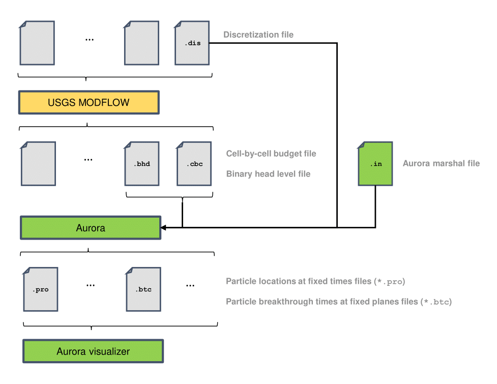
Aurora integrates tightly with MODFLOW-2005, which is still actively maintained by USGS; it is not designed to work with the rewritten MODFLOW 6. Aurora can directly parse MODFLOW-2005’s binary-format output files for cell-by-cell water budget (*.cbc) and hydraulic head (*.bhd), as well as its human-readable discretization (*.dis) file. Along with one additional Aurora-specific input file, called the marshal file, these provide all the information that Aurora needs to perform its simulations.

The sequence of steps required to generate useful results is the following, summarized in Figure 6:

• 1. Set up the MODFLOW model and run MODFLOW. This guide will not discuss how to do this in detail, but a convenient, free tool for this purpose is USGS ModelMuse (Aurora can read ModelMuse’s domain location and angle annotations directly from the *.dis file). You may use other front ends of your choosing: as long as Aurora can parse the *.dis file and the MODFLOW output, it does not matter what you use.

• 2. Set up the marshal (input) file for Aurora. This is a single, human-readable plain text file that contains all the information Aurora needs to run a simulation, with the exception of that which was computed by MODFLOW. Aurora will need to know the names of the MODFLOW discretization file (*.dis), budget file(s) (either MODFLOW *.cbc or GW Chart *.f* files), and (optional) hydraulic head file (*.bhd). You specify these file names in the marshal file, and the files themselves must reside in the same directory as the marshal file. You also need to specify additional physics for the particle tracker, particle release sources, and desired output (see Section 4 for complete details). Complete discretization information must be found within the *.dis file. MODFLOW supports scenarios in which the discretization file merely lists FORTRAN file unit numbers of separate files containing the discretization information. However, this is not supported by Aurora.

• 3. Open a console (e.g., Command Prompt or Windows Terminal), and navigate to the directory containing the Aurora executable. Run Aurora from the command line using the syntax:

    Aurora.exe <path to marshal directory> <name of marshal file>
  

  On non-Windows platforms, use the name of the executable complied for your architecture, for example

      ./aurora-linux-x64 <path to marshal directory> <name of marshal file>
  

  Throughout this document, the angle bracket notation is used to indicate the description of an argument. You must substitute in the relevant quantity in the marshal file; do not type the angle brackets or the text within them. If the marshal file is named Marshal.txt, its name can be omitted; just specify the directory that contains it and the other input files. Note that if there are spaces in , you will have to put quotation marks around it. Aurora will create individual output files within the marshal directory for each of the breakthrough surfaces (*.btc) and each of the profile times (*.pro) you specify in the marshal file. These list, respectively, individual particle breakthrough times and individual particle locations.

• 4. The output files are in human-readable text format and may be used with a post-processor of your choice, including Microsoft Excel or Mathworks MATLAB. Alternatively, Aurora comes with a number of Python visualization scripts, collectively known as the Aurora Visualizer. These are described in Section 3.2.

3.2 Visualization

Aurora ships with a number of Python scripts that use the Matplotlib library to perform visualization. These work without modification, but will generally need to be modified as needed, or used as templates for your own analyses. At the very least, you will need to alter the scripts to reference the locations of your analysis files, as these are hard-coded in the scripts. You may also want to alter the scripts more deeply to suit your own projects: this is possible with basic knowledge of the Numpy, Scipy, and Matplotlib Python packages. The scripts included in the Visualizer directory are:

VisBTC.py

Generates a plot of breakthrough curve (expressed as a relative concentration) by performing kernel density estimation on the arrival times in a single .btc file.

VisPlumeMapFrame.py

Generates a colour map of the depth-integrated concentration in the \(x\)-\(y\) plane by performing kernel density estimation on the particle locations in a single .pro file.

VisPlumeMapMovie.py

Calls VisPlumeMapFrame.py on each .pro file and stitches the frames together into an animation.

VisSideMapFrame.py

Same as VisPlumeMapFrame.py, but provides a depth-integrated view in the \(x\)-\(z\) plane.

Vis3DSwarmFrame.py

Plots the particle locations in a single .pro file on 3D isometric axes, showing the row, column, and layer discretization in the .dis file.

Vis3DSwarmMovie.py

Calls Vis3DSwarmFrame.py on each .pro file and stitches the frames together into an animation.

Some examples in the Examples directory also contain custom Python analysis scripts that may be useful as templates for your own analyses.

4 Specifying the Aurora marshal (input) file

4.1 Overview

As mentioned, all that is necessary to define an Aurora model is to correctly specify the contents of the marshal file is divided into blocks that begin with a capitalized keyword: MAIN, DOMAIN, LAYER, SPECIES, DECAY, MIMT_ADJUSTMENT, BREAKTHROUGHS, PROFILES, MOLAR_SOURCE, or SOURCE and end with the keyword END. The marshal file must begin with exactly one MAIN block, describing the non-physics details of the simulation. The additional physics defining the parameters and pdf’s mentioned in Section 5 must also be specified for each layer. This may be done for all layers at once using a single DOMAIN block, and/or for individual layers with individual LAYER blocks. After these initial blocks, any number (including zero) of each of the other types of blocks may be listed in any order.

Blocks are parsed by position, top to bottom, with one definition (generally a single number or string) per line, with preceding white space and trailing comments ignored. The interpretation given by Aurora to the entry on a given line is determined by its distance from the top of the block. The sole exception to this parsing rule is that there may be variable-length sub-blocks within a block: sub-blocks define simulation features for which the user may pick from alternatives where different alternatives require different numbers of parameters. Sub-blocks are each understood to only occupy one line of their parent block for the purposes of positional parsing of the parent. Sub-blocks may occupy multiple lines, in which case they are themselves parsed by position in the same way that blocks are (but terminating with ESB, not END. A multi-line sub-block looks like this:

      SUBBLOCK_NAME
        <argument 1> <optional, ignored comment>
        <argument 2> <optional, ignored comment>
        ...
      ESB

At your discretion, with no functional difference, a sub-block may be written inline, with its name followed by -> and multiple space-delimited entries and generally no comment allowed (unless a sub-block has a fixed number of entries, in which case additional text is ignored).

      SUBBLOCK_NAME -> <argument 1> <argument 2> ...

In cases where a sub-block has an indefinite number of arguments, each of which is defined by more than one number or string (for example when defining a molar concentration source, there will be multiple epochs, each defined by a start time and a concentration), the constituent tokens (space-delimited strings or numbers) of the argument are grouped by square brackets, and are collectively called a tuple. Each tuple is treated as a single argument, and may be followed by a comment in multi-line format. For example:

   SUBBLOCK_NAME
     [<argument 1, token 1> <argument 1, token 2>] <optional, ignored comment>
     [<argument 2, token 1> <argument 2, token 2>] <optional, ignored comment>
     ...
   ESB

4.2 Main block

The main block defines global information about the simulation. The first line contains the name of the discretization file. Next is a sub-block indicating whether Aurora should calculate velocities using only the portions of cells below the water table, or if it should assume all cells are saturated. This sub-block will either simply be the keyword ASSUME_SATURATED, or it will have the form

      BHD_FILE -> <name of binary head file>

Next, a sub-block specifies the files containing water budget information. MODFLOW *.cbc files can now be read directly, so the recommended form of this is:

      CBC_FILE -> <name of MODFLOW cell-by-cell water budget binary file>

For compatibility with old versions of Aurora, human-readable budget information produced from the MODFLOW *.cbc files by GW Chart can still be used. In this case, the budget sub-block has the format:

      GW_CHART_FILES
        <flow front face file>
        <flow right face file>
        <flow lower face file>
      ESB

If one of these face flow files is not needed because the model is only one cell thick in the appropriate direction, then NONE can be entered on the appropriate line of the GW_CHART_FILES sub-block. On the next line after the sub-block, the step length, \(d\) is defined, and then on the next line, the maximum time of the PT simulation is given. Next comes the grid-offset sub-block. This may simply be the token AUTO_GRID_OFFSET, in which case Aurora looks for global coordinates of the lower left corner of the grid and grid angle in ModelMuse-provided comments at the top of the .dis file. If it does not find them, it assumes zero offset and angle. Alternatively, one may manually specify these quantities with a sub-block of the following form:

      MANUAL_GRID_OFFSET
        [<x' offset> <y' offset>]
        <grid angle in degrees>
      ESB

A final sub-block, MOLES_PER_PARTICLE, is required if any MOLAR_SOURCE blocks are in the input file, and is optional (and ignored) otherwise.

Here is an example main block for a 1D system which only features one flux file:

   MAIN
     tce_decay.dis               MODFLOW geometry discretization file name
     ASSUME_SATURATED
     CBC_BUDGET -> tce_decay.cbc
     1.0                         Spatial length of each step along streamline [L]
     2e8                         Maximum time of simulation [T]
     AUTO_GRID_OFFSET
     MOLES_PER_PARTICLE -> 1e-6
   END

4.3 Domain and layer blocks

All the information about the additional small-scale physics must be defined for each layer of the model, this can be done for all layers at once using a DOMAIN block or for a specific layer using LAYER <#> block, where <#> represents the index of the layer being defined, with layer 0 being the bottom layer of the model. An unlimited number of these blocks can be used, with blocks later in the marshal file redefining parameters defined in earlier blocks where these conflict. The syntax inside either type of block is the same: The first line contains the porosity, \(\theta \ \mathrm {[-]}\). Next comes the transverse dispersivity sub-block, which defines the values of the local-scale horizontal transverse dispersivity, \(\alpha _h\ \mathrm {[L]}\), and vertical transverse dispersivity, \(\alpha _v\ \mathrm {[L]}\). This sub-block can be either NONE, if transverse dispersive physics is not desired, or written as:

      TRANSVERSE_DISP -> <horizontal dispersivity>   <vertical dispersivity>

Next comes one advective heterogeneity sub-block, which contains the parameters defining \(f(r)\) and which may be of any of the types introduced in the theory section. The syntax of each type of sub-block is listed in inline form (select only one):

NONE:

indicating pure tracing the large-scale streamlines, as per (12)

ADE -> <\(\alpha _l\)>:

indicating advective-dispersive (Fickian) small-scale behavior, defined by a single user-defined parameter, \(\alpha _l\ \mathrm {[L]}\), representing longitudinal dispersivity. This corresponds to distribution (13).

LOGNORMAL -> <\(\sigma ^2\)>:

indicating mildly heavy-tailed breakthrough where the pdf for \(r\) is defined by a single log-variance, \(\sigma ^2 \ \mathrm {[-]}\). This corresponds to distribution (14).

PARETO -> <\(\beta \)>:

indicating a heavy-tailed advective breakthrough with a pure power law tail that is defined by a single parameter, \(\beta \ \mathrm {[-]}\). This corresponds to distribution (15).

TPL -> <\(r_2/r_1\)> <\(\beta \)> :

indicating a truncated (or tempered) power law, where the parameters are as shown in (16). The ratio of \(t_2:t_1\) is user-selectable and Aurora solves form the actual values that make \(f(r)\) have unit mean.

Finally comes the MIMT sub-block, which defines \(\lambda \) and \(g(t)\), if relevant. Again, the syntax of each type of sub-block is listed in inline form, followed by its mathematical definition. Three options are available (select only one):

NONE:

indicating no immobilization at all, so neither \(\lambda \) nor \(g(t)\) need to be specified.

EXPONENTIAL -> <\(\lambda \)> <\(\mu \)>:

indicating immobilization rate \(\lambda \ \mathrm {[T^{-1}]}\), and immobilization time pdf

\(\seteqnumber{0}{}{2}\)

\begin{equation} g(t)=\mu e^{-\mu t}, \end{equation}

where \(\mu \ \mathrm {[T^{-1}]}\) is an arbitrary, user-defined rate constant.

TPL -> <\(\lambda \)> <\(t_1\)> <\(t_2\)> <\(\beta \)>:

indicating immobilization rate \(\lambda \) and truncated power law immobilization time pdf, with a slightly different definition from that used for small-scale advective heterogeneity:

\(\seteqnumber{0}{}{3}\)

\begin{equation} g(t) \propto \left (1+\frac {t}{t_1}\right )^{-1-\beta }e^{-\frac {t}{t_2}}, \end{equation}

The TPL definition here is based on the shifted Pareto distribution, and so has support on the whole half line \([0,\infty )\), and any positive values of the exponent, \(\beta \ \mathrm {[-]}\), scaling time, \(t_1\ \mathrm {[T]}\), and truncation time, \(t_2\ \mathrm {[T]}\), are permitted.

Example of a domain block:

      DOMAIN
        0.25              Assumed porosity
        TRANSVERSE_DISP
          1e-1            Horizontal transverse dispersivity [L]
          1e-1            Vertical transverse dispersivity [L]
        ESB
        PARETO -> 1.2     Beta [-]
        EXPONENTIAL
          4e-4            Immobilization rate [T^-1]
          5e-4            Remobilization rate [T^-1]
        ESB
      END

Example of an individual layer declaration for layer index 1: second from the bottom of the domain. Here, only MIMT physics are operative; there is no advective scattering of any sort:

   LAYER 1
     0.3            Assumed porosity
     NONE           Sub-grid transverse dispersivity [L]
     NONE           Advective heterogeneity block
     EXPONENTIAL
       1e-4
       5e-5
     ESB
   END

4.4 Species block

It is possible for Aurora to keep track of different aqueous chemical species, which can be assigned to different sources, which can participate in first-order decay networks (discussed below) with species-specific decay rates, and which feature species-specific MIMT behavior. Two special species are always defined without needing an explicit declaration: Default, which is a species that (by default) does not decay and has unmodified MIMT behavior, and Null, which is permanently immobile and does not undergo decay. Null can be specified as a destination species in a decay network, and has the effect of eliminating mass from the simulation.

To define additional chemical species, their names must be listed in the optional SPECIES block, with each line beginning with exactly one species name. Species names are not case sensitive, and may not contain spaces; all text after the first word on each line is treated as a comment. If no species besides Default and Null are used in the simulation, then it is not necessary to include a SPECIES block.

Here is an example of a species block, listing the names of three chlorinated solvent species:

   SPECIES
     TCE
     DCE
     VC
   END

4.5 Decay block

The decay behavior outlined in Section 5.4.2 is specified in the optional DECAY block. This block contains an arbitrary number of sub-blocks, with each having the format:

  <source species>
    <decay rate>
    [<daughter species 1> <daughter species 1 moles per source mole>]
    [<daughter species 2> <daughter species 2 moles per source mole>]
    ...
  ESB

Here the <source species> name must either be Default, or a species that was defined in a previous SPECIES block. The <decay rate> defines the first-order rate constant for a given decay reaction. Next come one or more tuples, [<daughter species name> <daughter species moles per source mole>], specifying the number of moles of each daughter species produced by decay of one mole of <source species>. Each daughter species must be Null or one of the species that has been listed in a previous SPECIES block. Arbitrary decay networks are permitted, and it is permissible for the same species to appear as the source for multiple sub-blocks, and also as the destination in multiple sub-blocks. Where a one-mole-to-one-mole decay relation exists, a simpler sub-block format is permitted:

  <source species> -> <decay rate> <daughter species>

Here is an example of kinetics specification for a straight chlorinated solvent decay chain.

   DECAY
     TCE -> 1.456e-8 DCE
     DCE -> 1.68e-8 [VC 1]
     VC -> 1.36e-8 Null
   END

4.6 MIMT adjustment block

The species-specific rescaling factors discussed in Section 5.4.1 are presented in the optional MIMT_ADJUSTMENT block. Any species \(S\) that does not use the unmodified \(\lambda \) and \(g(t)\) MIMT parameters can have its rescaling factors listed explicitly, in its own sub-block. The format of each line in the block is:

  <species> -> <immobilization factor> <remobilization factor>

where <species> is the name of a species \(S\) previously listed in the SPECIES block, <immobilization factor> is \(\tau _S^{im}\), and <remobilization factor> is \(\tau _S^{m}\).

Here is an example of an MIMT adjustment block, which rescales the mobile and immobile times used to compute the clock time for two species:

   MIMT_ADJUSTMENT
     TCE -> 4 1
     VC -> 1.5 1
   END

4.7 Source block

There are two types of source blocks supported by Aurora: MOLAR_SOURCE blocks, which represent time-varying specified concentration or specified-flux sources, and the more primitive SOURCE blocks which simply inject a specified number of particles, regardless of the MOLES_PER_PARTICLE setting in the MAIN block.

4.7.1 Raw particle sources

Any number of SOURCE blocks may be employed, each defining a source of particles. On the first line, the total number of particles to be released from the source is specified. Next is a sub-block representing the release regime, which may be INSTANT -> —all particles released at —or CONTINUOUS -> , with all particles released at uniformly-distributed random times between and .

On the next line, a selection is made as to whether particles should be randomly spatially distributed throughout the source region (UNIFORMLY_WEIGHTED) or if their spatial distribution within the region should be proportional to the groundwater speed (FLUX_WEIGHTED).

Next there is one sub-block defining the source region itself. Options for each source region sub-block are (select only one):

BOX -> <\(x_\mathrm {min}\)> <\(x_\mathrm {max}\)> <\(y_\mathrm {min}\)> <\(y_\mathrm {max}\)> <\(z_\mathrm {min}\)> <\(z_\mathrm {max}\)>:

defining a source in which particles are introduced uniformly randomly into the interior of the box-shaped spatial region \(x_\mathrm {min}<x<x_\mathrm {max} \cap y_\mathrm {min}<y<y_\mathrm {max} \cap z_\mathrm {min}<z<z_\mathrm {max}\).

CYLINDER -> <\(x_\mathrm {mid}\)> <\(y_\mathrm {mid}\)> <\(z_\mathrm {min}\)> <\(r\)> <\(h\)>:

defining a source in which particles are introduced uniformly randomly into the interior of the truncated cylinder of radius \(r\) whose axis is parallel to the \(z\)-axis and intersects the \(x\)-\(y\) plane at \((x_\mathrm {mid},y_\mathrm {mid})\), with \(z\)-coordinates in the interval \((z_\mathrm {min},z_\mathrm {min}+h)\).

TUBE -> <\(x_\mathrm {mid}\)> <\(y_\mathrm {mid}\)> <\(z_\mathrm {min}\)> <\(r\)> <\(h\)>:

defining a source in which particles are introduced uniformly randomly only onto the outer curved surface of the truncated cylinder of radius \(r\) whose axis is parallel to the \(z\)-axis and intersects the \(x\)-\(y\) plane at \((x_\mathrm {mid},y_\mathrm {mid})\), with \(z\)-coordinates in the interval \((z_\mathrm {min},z_\mathrm {min}+h)\).

SPHERE -> <\(x_\mathrm {mid}\)> <\(y_\mathrm {mid}\)> <\(z_\mathrm {mid}\)> <\(r\)>:

defining a source in which particles are introduced uniformly randomly into the interior of a sphere of radius \(r\) whose centre is at \((x_\mathrm {mid},y_\mathrm {mid},z_\mathrm {mid})\).

After the geometry sub-block, there is an optional sub-block specifying the species defined in the source (only one species is defined in the source), of the form SPECIES -> , where was listed previously in the SPECIES block. If no species sub-block is specified, then the Default species is assumed. Even if first-order decay behavior is specified for the species and the source is continuous, no decay is assumed to occur before the particle is introduced into the domain.

   SOURCE
     10000            Number of particles to employ [-]
     INSTANT -> 0.0   Time of instantaneous release [T]
     FLUX_WEIGHTED
     TUBE -> 27.5 -27.5 -10 0.1 10
   END

4.7.2 Molar sources

     FIXED_CONC
       [<start time of epoch 1 [T]> <molar concentration during epoch 1 [-]>]
       [<start time of epoch 2 [T]> <molar concentration during epoch 2 [-]>]
       ...
     ESB

or

   FIXED_RATE
     [<start time of epoch 1 [T]> <molar injection rate during epoch 1 [T^-1]>]
     [<start time of epoch 2 [T]> <molar injection rate during epoch 2 [T^-1]]>]
     ...
   ESB

Next, there is a sub-block indicating the inactivation time of the source. In the case of a fixed concentration type of source, this represents the time after which the number of particles in the source is not maintained, and the source region is treated as any other region in the domain. For a specified injection rate, this represents the end of the final epoch of injections. In both cases, the syntax for the sub-block is END_TIME -> .

Next there is one sub-block defining the source region itself. Options for this sub-block (select only one) are:

BOX -> <\(x_\mathrm {min}\)> <\(x_\mathrm {max}\)> <\(y_\mathrm {min}\)> <\(y_\mathrm {max}\)> <\(z_\mathrm {min}\)> <\(z_\mathrm {max}\)>:

defining a source in which particles are introduced uniformly randomly into the interior of the box-shaped spatial region \(x_\mathrm {min}<x<x_\mathrm {max} \cap y_\mathrm {min}<y<y_\mathrm {max} \cap z_\mathrm {min}<z<z_\mathrm {max}\).

CYLINDER -> <\(x_\mathrm {mid}\)> <\(y_\mathrm {mid}\)> <\(z_\mathrm {min}\)> <\(r\)> <\(h\)>:

defining a source in which particles are introduced uniformly randomly into the interior of the truncated cylinder of radius \(r\) whose axis is parallel to the \(z\)-axis and intersects the \(x\)-\(y\) plane at \((x_\mathrm {mid},y_\mathrm {mid})\), with \(z\)-coordinates in the interval \((z_\mathrm {min},z_\mathrm {min}+h)\).

SPHERE -> <\(x_\mathrm {mid}\)> <\(y_\mathrm {mid}\)> <\(z_\mathrm {mid}\)> <\(r\)>:

defining a source in which particles are introduced uniformly randomly into the interior of a sphere of radius \(r\) whose centre is at \((x_\mathrm {mid},y_\mathrm {mid},z_\mathrm {mid})\).

Finally, there is a mandatory sub-block specifying the species defined in the source (only one species is defined in a given MOLAR_SOURCE), of the form SPECIES -> , where was listed previously in the SPECIES block or is Default.

   MOLAR_SOURCE
     FIXED_CONC
       [0.0 1e-7]      <Epoch start [T]> <Concentration [1/L^3]>
     ESB
     END_TIME -> 2e7   Source inactivation time [T]
     BOX
       5               Release box: Minimum X [L]
       6               Release box: Maximum X [L]
       -100            Release box: Minimum Y [L]
       0               Release box: Maximum Y [L]
       -10             Release box: Minimum Z [L]
       0               Release box: Maximum Z [L]
     ESB
     SPECIES -> TCE
   END

4.8 Breakthroughs block

Any number of BREAKTHROUGHS blocks may be employed, although there is generally no reason for more than one to be used. There may be any number of sub-blocks in a BREAKTHROUGHS block, each defining the geometry of a 2D surface at which particle crossing times are to be recorded, as well as a crossing direction required to trigger a breakthrough , which may be IN, OUT, or EITHER. All surfaces are defined by some equation \(h(\bm {x})=C\), where \(C\) is a scalar constant, and an IN transition is defined as one where \(h(\bm {x}_{n+1}) < C < h(\bm {x}_{n})\), where \(\bm {x}_{n}\) represents the particle’s position after the \(n\)-th step. An OUT transition is defined conversely. Two types of breakthrough sub-blocks may be defined (specify as many as you like):

TUBE -> <\(x_\mathrm {mid}\)> <\(y_\mathrm {mid}\)> <\(z_\mathrm {min}\)> <\(r\)> <\(h\)> :

defining a surface identical to that defining the TUBE source discussed above. When = IN, particle motion is towards the axis of the cylinder.

PLANE -> <\(a\)> <\(b\)> <\(c\)> <\(d\)> :

defining a planar surface of infinite extent defined by the equation \(ax+by+cz-d=0\).

Here is an example breakthrough block which triggers an event whenever a particle passes into a tubular shell. This formulation might be used to model breakthrough of solute returning to a well during a push-pull test.

  BREAKTHROUGHS
    TUBE -> 27.5 -27.5 -10 0.1 10 IN
  END

4.9 Profiles block

Any number of PROFILES blocks may be employed, although there is generally no reason for more than one to be used. There may be any number of lines in a given PROFILES block, each containing a time at which locations of all active particles (those which have not previously reached a stagnation point) should be recorded.

  PROFILES      Times at which particle snapshots are desired
    5e6
    5e7
    1.0e8
    2.0e8
  END

5 Detailed theory

5.1 The CTRW-on-a-streamline particle tracking algorithm

We will introduce the algorithm by building up systematically from simple streamline-tracing particle tracking algorithm, similar to that found in MODPATH or other programs. A classic particle tracking algorithm that just follows streamlines would have a user-specified step size in either space or time. If \(\Delta _t\ \mathrm {[T]}\) is fixed, the model is as simple as possible.

\begin{eqnarray} \bm {x}_{n+1} &=& \bm {x}_n + \bm {v}(\bm {x}_n) \Delta _t \label {eq: pure adv}\\ t_{n+1} &=& t_n + \Delta _t \label {eq: time update} \end{eqnarray}

Alternatively, purely advective streamline tracking could be implemented using fixed travel distance, \(d\), with an operational time increment, \(\Delta _{t_O}\ \mathrm {[T]}\), recalculated on every step, \(n\):

\begin{eqnarray} \bm {x}_{n+1} &=& \bm {x}_n + \frac {\bm {v}(\bm {x}_n)}{\| \bm {v}(\bm {x}_n) \|}d \\ t_{O,n+1} &=& t_{O,n} + \Delta _{t_O,n}. \end{eqnarray}

To add small scale flow-field variability, we need to separate \(\Delta _{t_O,n}\), due to Darcy-scale advection (the only thing visible in a MODFLOW model), and a \(\Delta _{t_A}\), including all advection. Each segment of length \(d\) of a large-scale streamline may be conceptualized as representing a flux-weighted ensemble, or “bundle”, of small-scale, adjacent stream tubes of length \(d\) with varying local harmonic mean hydraulic conductivity. Each small-scale stream tube has a different advection time, \(\Delta _{t_A}\), and because the small-scale stream tubes in an ensemble are epistemically interchangeable (we have no knowledge of their exact position or of the particular small-scale tube to which a particle being tracked along a large-scale streamline belongs), it is sensible to define a conditional probability distribution, \(\phi (\Delta _{t_A}|\Delta _{t_O})\).

The nature of \(\phi (\Delta _{t_A}|\Delta _{t_O})\) can be characterized by noting that the small-scale stream tubes in an ensemble share approximately the same gradient: justified by the fact that the global head field is an integral quantity and is smooth relative to the underlying hydraulic conductivity (\(K\)) field. Because \(K\ \mathrm {[LT^{-1}]}\) is everywhere independent of the boundary conditions on head that determine the magnitude of the large-scale effective \(\bm {v}\), and the head drop is shared by small-scale stream tubes in an ensemble, it follows that the Darcy velocities in each of the tubes in the ensemble always maintain a same constant of proportionality to \(\|\bm {v}\|\), regardless of system boundary conditions. And because \(d\) is fixed, the same is true of travel time, \(\Delta _{t_A}\). Thus a simple scaling law applies: \(\phi (\Delta _{t_A}|\Delta _{t_O})\Delta _{t_O}=\phi (\Delta _{t_A}/\Delta _{t_O}|1)=:f(r)\), where \(f\) is some unknown pdf, solely determined by the statistics of small-scale heterogeneity, which contains all relevant information for mapping from operational time to true advection time, and \(r=\Delta _{t_A}/\Delta _{t_O}\). This informal argument is supported by a number of lines of evidence from the academic literature, and by extension of advective-dispersive behavior, which can be expressed in terms of \(d\) and \(r\) alone, as in (13).

To add any MIMT, whether due to diffusion into secondary porosity or due to chemical adsorption, we define two additional probability distributions. The first one is exponential, with a rate constant, \(\lambda \), representing the probability of immobilization of mobile solute per unit time traveled. The second, not necessarily exponential, distribution, \(g(t)\), represents the time for the length of a single particle immobilization event. The exponential form of the mobile-time distribution is justified by the assumption of randomly located sites that are dense relative to length scale \(d\). We note that the \(\lambda \) and \(g\) approach captures even multiple types of immobilization sites with different capture and release distributions (i.e. multi-rate mass transfer), as the time until the first event for multiple simultaneous exponentially-distributed processes is itself exponential, and we can create an immobilization-site-prevalence-weighted average of the immobilization time pdf’s for the various site types.

To quantify the travel time increase due to MIMT, we can develop a conditional pdf, \(\zeta (\Delta _{t}|\Delta _{t_A})\). We note that the total (clock) time is the advection time, \(\Delta _{t_A}\) plus the delay due to \(n\) independent immobilization events each of whose lengths is drawn from \(g(t)\). The probability mass function for \(i\) immobilization events, \(w(i)\ \mathrm {[-]}\), is Poisson distributed with parameter \(\lambda \Delta _{t_A}\)

The last complication is added to allow hopping between streamlines via small-scale transverse dispersion in the plane transverse to the streamline. Aurora allows definition of horizontal and vertical transverse dispersion, where both dispersion directions are orthogonal to the local flow velocity, \(\bm {v}\), and to each other. In addition, the horizontal dispersion is defined to be in the plane orthogonal to \(\bm {k}\), the unit vector in the \(z\)-direction. To generate the horizontal and vertical dispersion unit vectors, \(\bm {n}_h\) and \(\bm {n}_v\) the following cross-product expressions are employed:

\begin{eqnarray} \bm {n}_h &=& \frac {\bm {k} \times \bm {v}(\bm {x})}{\|\bm {k} \times \bm {v}(\bm {x}) \|_2} \label {eq: n1}\\ \bm {n}_v &=& \frac {\bm {n}_h \times \bm {v}(\bm {x})}{\|\bm {n}_h \times \bm {v}(\bm {x}) \|_2} \label {eq: n2} \end{eqnarray}

The size of the horizontal transverse dispersive motion is defined by performing a random draw \(\eta _h \sim \mathcal {N}(0,2 \alpha _h d)\), where \(\alpha _h\) represents the horizontal transverse dispersivity. Similarly, the size of the vertical transverse dispersive motion is defined by performing a random draw \(\eta _v \sim \mathcal {N}(0,2 \alpha _h d)\), where \(\alpha _v\) represents the vertical transverse dispersivity Finally, the perturbation between streamlines is computed:

\begin{eqnarray} \Delta _{\bm {x},n} = \eta _h\bm {v}_h + \eta _v\bm {v}_v. \end{eqnarray}

5.2 Modelling advective heterogeneity in Aurora

As indicated, spreading due to local-scale scattering is treated in Aurora by defining the probability distribution function \(f(r)\), where \(r\) is the ratio of actual advection time, incorporating small-scale advective heterogeneity, to the notional advection time based on the MODFLOW-derived deterministic large-scale velocity field. The choice of this function depends on on the physics to be modelled, and on the needs of the user.

5.2.1 Purely advective streamline tracing

Pure streamline tracing, as in MODPATH, can be achieved by use of a shifted Dirac delta distribution:

\begin{equation} f(r)=\delta (r-1) \label {eq: shifted delta} \end{equation}

Here particles simply travel along the large-scale deterministic streamlines determined from MODFLOW at the velocity implied by Darcy’s law. Such an approach might be indicated if MIMT were the dominant process, but usually there are better options.

5.2.2 Classical advection and dispersion

Classical-advection dispersion can be modelled by use of the following definition (based on the so-called Inverse Gaussian distribution):

\begin{equation} f(r)=\frac {1}{r\sigma \sqrt {2\pi }}\exp \left \{-\frac {(\ln r+\sigma ^2/2)^2}{2\sigma ^2}\right \} \label {eq: lognormal}. \end{equation}

The log-normal distribution is a two-parameter distribution, but the requirement that mean flow velocity is unchanged by the small-scale heterogeneity imposes the condition \(\mathrm {E}[r]=1\) and constrains the log-mean. Empirically, for a long variance below about 0.5, the Log-normal distribution is essentially identical to the Inverse Gaussian with the same mean and variance (this is to say, it describes Fickian behaviour).

Pareto distributions may be employed to model heavy-tailed advective breakthrough with a pure power law tail, and are defined by a single parameter, \(\beta \ \mathrm {[-]}\), which represents the power law exponent:

\begin{equation} f(r) = \beta ^{1-\beta }(\beta -1)^\beta r^{-(\beta +1)} \label {eq: pareto}. \end{equation}

As elsewhere, the constraint \(\mathrm {E}[r]=1\) removes one degree of freedom from the standard Pareto distribution. Values of \(\beta < 1\) yield a distribution with infinite mean and variance and persistently non-Fickian tailing. Such a choice recovers the time-fractional ADE within Aurora.

Truncated power law (TPL) distributions are perhaps the most popular choice for capturing non-Fickian subsurface transport, and represent a Pareto distribution with exponential tempering at late time. As all TPL moments are finite, the transport behaviour they describe eventually becomes Fickian, although not necessarily over time scales of interest. It is implemented in Aurora as an advection time PDF, via the equation

\begin{equation} f(r) \propto \left (\frac {r}{r_1}\right )^{-1-\beta }e^{-\frac {r}{r_2}} \label {eq: TPL}, \end{equation}

using the three dimensionless parameters \(r_1\), \(r_2\), and \(\beta \). \(r_2\) represents the onset time of the exponential tapering. Note that (16) is shown as a proportionality relationship rather than an equality. For any specified \(r_2/r_1\) and \(\beta \), Aurora solves for \(r_1\) and \(r_2\) that enforces the constraint \(\mathrm {E}[r]=1\).

5.3 Modelling mobile-immobile mass transfer (MIMT) in Aurora

The formulation of MIMT used by Aurora corresponds to an Eulerian transport equation of the form

\begin{equation} \frac {\partial c_\mathrm {m}}{\partial t} + \lambda c_\mathrm {m} - \int _{0}^{t} g(t-\tau ) \lambda c_\mathrm {m}(\tau ) d\tau = L\left \{c_\mathrm {m}\right \}, \label {eq: our MIMT} \end{equation}

where \(L\) is a linear transport operator, and we use \(c_\mathrm {m}\) to refer explicitly to the mobile concentration. This differs superficially from many of the approaches to MIMT in the literature, so it is necessary to outline how this relates to them, and how \(\lambda \) and \(g(t)\) may be determined explicitly from the parameters defining other MIMT formulations seen in the literature. We consider three such cases in the next subsections.

5.3.1 Coding multi-rate mass transfer (MRMT)

MRMT is a formulation that obviously generalizes single-rate mass transfer, but also dual-porosity models, explicit models of diffusion into secondary structures such as slabs, spheres, and cylinders, and slow kinetic sorption. The general MRMT transport equation has the form

\begin{equation} \frac {\partial c_\mathrm {m}}{\partial t} + \frac {\partial c_\mathrm {im}}{\partial t} = L\left \{c\right \}, \label {eq: normal MIMT} \end{equation}

and needs to be closed by means of a relationship between \(c_\mathrm {im}\) and \(c_\mathrm {m}\). This relationship is most commonly expressed as a convolution,

\begin{equation} \frac {\partial c_\mathrm {im}}{\partial t} = G*\frac {\partial c_\mathrm {m}}{\partial t}, \label {eq: standard im-m relation} \end{equation}

where \(G(\cdot )\) is a “memory function”. We may integrate by parts to yield

\begin{equation} \frac {\partial c_\mathrm {im}}{\partial t} = G(0)c_\mathrm {m}(t) - \cancelto {0}{G(t)c_\mathrm {m}(0)} + \frac {\partial G}{\partial t}*c_\mathrm {m}. \label {eq: standard im-m final} \end{equation}

The canceled term arises from the fact that (19) is derived for an initially zero-concentration domain. An apparently different formulation relating the immobile concentration to the mobile concentration is also seen in the literature:

\begin{equation} c_\mathrm {im} = \int _0^t G(t-\tau )c_\mathrm {m}(\tau )d\tau . \label {eq: dentz im-m relation} \end{equation}

However, when differentiated with respect to \(t\), it yields

\begin{equation} \frac {\partial c_\mathrm {im}}{\partial t} = G(0)c_\mathrm {m}(\tau ) + \frac {\partial G}{\partial t}*c_\mathrm {m}, \label {eq: dentz im-m final} \end{equation}

which is consistent with (20). From inspection of either (20) or (22), it is obvious that the definitions

\begin{eqnarray} \lambda &\equiv & G(0), \label {eq: MRMT-CTRW equivalence lambda}\\ g(t) &\equiv & \frac {\partial G}{\partial t}, \label {eq: MRMT-CTRW equivalence g} \end{eqnarray}

make (17) equivalent to (18) combined with (19).

5.3.2 Coding first-order mass transfer

First-order mass transfer is described by the governing equation

\begin{equation} \frac {\partial c_\mathrm {m}}{\partial t} + \mu (c_\mathrm {im}-c_\mathrm {m}) = L\left \{c_\mathrm {m}\right \}. \label {eq: first-order MIMT} \end{equation}

While this is plainly a special case of single rate mass transfer with equal rate constants for both immobilization and remobilization, and this is itself a subset of MRMT, there is no memory function in this formulation, and so separate analysis is required to derive \(\lambda \) and \(g(t)\). We note that if we define \(g(t)=\mu \exp (-\mu t)\), then the probability of a particle remaining immobile for at least \(T\) is \(\int _T^\infty \mu \exp (-\mu t) dt = \exp (-\mu T)\). The immobile concentration at time \(t\) is the integral of the mobile-immobile flux at each previous time, \(\tau \), weighted by the probability of remaining immobile for at least \(T=t-\tau \). Thus, it follows that

\begin{eqnarray} c_\mathrm {im} &=& \int _{0}^{t} e^{-\mu (t-\tau )} [-\lambda c_\mathrm {m}(\tau )] d\tau ,\\ -\mu c_\mathrm {im} &=& \int _{0}^{t} g(t-\tau ) \lambda c_\mathrm {m}(\tau ) d\tau . \end{eqnarray}

It then follows from direct inspection that (17) and (25) are equivalent, as long as the following identification is made:

\begin{eqnarray} \lambda &\equiv & \mu , \label {eq: FO-CTRW equivalence lambda}\\ g(t) &\equiv & \mu e^{-\mu t}. \label {eq: FO-CTRW equivalence g} \end{eqnarray}

5.3.3 Translating from a retardation factor model

The final case we consider is a transport equation where MIMT is encoded by multiplication of the time derivative by a retardation factor, R:

\begin{equation} R\frac {\partial c_\mathrm {m}}{\partial t} = L\left \{c_\mathrm {m}\right \}. \label {eq: retardation MIMT} \end{equation}

We note that this model is an inherently defective simplification of first-order mass transfer. The defect lies in the fact that MIMT always causes dispersion which is erroneously disregarded by use of the retardation factor alone. The so-called “local equilibrium assumption” actually amounts to the assumption that dispersion due to MIMT is small relative to other sources of dispersion. Thus, our approach is to begin with a single-rate mass transfer model, and define its parameters so that its effective velocity corresponds to that of the retardation model, and its dispersion due to mass transfer is “small” in some sense. This can not be said to have less realism than (30), and can generate arbitrarily close behavior. We begin from a slightly generalized form of (25), with distinct mobilization and immobilization rates:

\begin{equation} \frac {\partial c_\mathrm {m}}{\partial t} + \mu c_\mathrm {im} - \lambda c_\mathrm {m} = L\left \{c_\mathrm {m}\right \}. \label {eq: first-order MIMT relaxed} \end{equation}

It is easy to show that an equivalent \(R\) for any \(\lambda \) and \(\mu \) is defined

\begin{equation} R = 1 + \frac {\lambda }{\mu }. \label {eq: retardation} \end{equation}

It has been similarly been shown that the effective late-time Fickian dispersion coefficient, \(D_\mathrm {eff}\), corresponding to the MIMT in (31) is

\begin{equation} D_\mathrm {eff} = \frac {\lambda \mu v^2}{(\lambda +\mu )^3}, \end{equation}

where \(v\) is the magnitude of the streamline advection velocity. Thus, for (17) to match (30), we must select \(\lambda \) and \(\mu \) in (31) to match \(R\), and so that \(D_\mathrm {eff}\) is sufficiently small. This is attainable because \(R\) fixes only the ratio of \(\lambda \) and \(\mu \), and their respective magnitudes can be scaled by any factor, \(k\), to scale \(D_\mathrm {eff}\) by the factor \(k^{-1}\). We can bring (17) and (30) into arbitrary close alignment by choosing sufficiently large \(\mu \) and making the following identification:

\begin{eqnarray} \lambda &\equiv & (R-1)\mu , \label {eq: retardation-CTRW equivalence lambda}\\ g(t) &\equiv & \mu e^{-\mu t}. \label {eq: retardation-CTRW equivalence g} \end{eqnarray}

5.4 Multi-species operation

The particle tracking approach in Aurora is well suited to modeling single aqueous chemical species that do not undergo interactions. Although Aurora does not support bi-molecular of geochemical reactions, it does support the use of multiple labeled species that have their own sources and participate in first-order decay networks with arbitrary complexity and stoichiometry, and which feature distinct MIMT behavior. These features allow Aurora to be used for a variety of radionuclide and organic contaminant transport problems.

5.4.1 Species-specific MIMT behavior

The general functional form of the MIMT model is defined on a layer-by-layer basis, or for the system as a whole, so each layer will share a single \(\lambda \) and \(g(t)\). However, in multi-species systems, it may be desirable to alter the MIMT behavior of the different species to reflect different mobilization and remobilization propensities, either due to different sorption affinities or different diffusivities. This can be done by rescaling time for the purposes of computing immobilization and remobilization times, on a species-by-species basis. This is to say that for each species, \(S\), two dimensionless time rescaling constants, \(\tau _S^\mathrm {im}\) and \(\tau _s^\mathrm {im}\), may be defined that are used when computing the number of immobilization events, \(i\), and duration of each given immobilization event, \(t_{im}\), during a given particle step \(n\):

\begin{eqnarray} i &\sim & \mathrm {Poisson}(\lambda \tau _S^{im} \Delta _{t_A,n})\\ t_{im} &\sim & g(\tau _S^m t_{im}) \end{eqnarray}

These species-specific alterations apply throughout the domain, and modify the layer-specific \(\lambda \) (note that scaling \(\Delta _{t_A,n}\) may also be thought of as scaling \(\lambda \)) and \(g(t)\) everywhere.

For example, using equation (32), species-specific retardation coefficients could be achieved by selecting an appropriate \(\tau _S^\mathrm {im}\) for each species, \(S\), and leaving \(\tau _S^\mathrm {m} = 1\) for all species.

5.4.2 First-order decay networks

Both first-order annihilation (\(S\rightarrow 0\)) and transformation (\(S\rightarrow D\)) reactions are supported. First-order decay implies that, in a small time increment, \(dt\), a particle of type \(S\) has probability \(\kappa _\mathrm {S\rightarrow D} dt\) of being transformed into a particle of type \(D\) (which may be a special “null” species, representing annihilation), and is described by an exponential survival time distribution with constant \(\kappa _\mathrm {S\rightarrow D}\ \mathrm {[T^{-1}]}\).

As a stochastic particle tracker, Aurora models the first-order decay by pseudo-randomly deciding whether a decay event has occurred for each particle during each time step, after it has computed \(\Delta _{t}\). For each destination species, \(D_i\), that a particle of species \(S\) may decay to, a time, \(T_\mathrm {S\rightarrow D_i}\), is drawn according to:

\begin{equation} T_\mathrm {S\rightarrow D_i} \sim \kappa _\mathrm {S\rightarrow D_i} \exp (-\kappa _\mathrm {S\rightarrow D_i} t). \end{equation}

If for all \(D_i\), \(T_\mathrm {S\rightarrow D_i} > \Delta _t\) (the clock time for the transition), then no decay event occurs. Otherwise, decay to the species \(D_i\) with the smallest \(T_\mathrm {S\rightarrow D_i}\) occurs.